Since the introduction of the GPT-3 large language model (LLM), a new deep learning paradigm called ‘prompt engineering’ has been gaining popularity. In this article, our 17 year old AI Singapore intern, Liew Wei Pyn, from NUS High School of Math and Science, implemented a solution for a paraphrasing downstream task using a technique called ‘Prompt Tuning’ to generate soft prompts with an OPT-1B3 (1 billion parameters) pre-trained model from Meta.
Table of Contents
- Introduction
- Prompt Tuning
- Soft Prompts
- Datasets
- Implementation
- HuggingFace Model Wrapper
- Training
- Results
- Scoring Metrics
- Visualisation
- Conclusion
Introduction
Open Pre-trained Transformer (OPT) models are a collection of open source decoder-only pre-trained transformers by Meta AI ranging from 125M to 175B parameters, with 175B showing comparable performance against Open AI’s GPT-3. Such large language models display remarkable performance in zero and few-shot tasks, which prompts a promising solution for many tasks due to its capability of coaxing a large model into solving tasks they were not explicitly trained to do.
The task that we are trying to accomplish is to prompt OPT models into paraphrasing sentences. The task of paraphrasing is traditionally a sequence-to-sequence task accomplished using encoder-decoder transformer architectures (such as BART). However, there is still some promise in leveraging the large pre-trained decoder-only models like OPT, whose capabilities to model natural language may overcome the architectural limitations.
However, throughout the course of this experiment, we only work with OPT1.3B, a much smaller variant of the OPT175B model. As such, the results will not be incredible, as a smaller model cannot grasp sufficient complexities of the task at hand.
Prompt Tuning
For example, in OpenAI’s GPT-3 playground, we can use different techniques such as in-context learning and chain-of-thought prompting. An excellent example of chain-of-thought prompting is provided by the aforementioned paper:


Soft Prompts
The concept of soft prompts was introduced by Lester et al. in the paper titled “The Power of Scale for Parameter-Efficient Prompt Tuning”, where they explored prepending learnable tokens to the inputs of frozen language models as such:
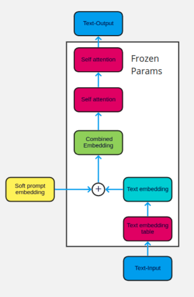
The learnable tokens are passing conceptual notions to the model in an attempt to better understand the task at hand. The models represent words as numbers in a high-dimensional space. As such, we need not restrict our prompts to discrete words, and are able to search in the space between words to find the most suitable prompts to feed into the model.
These prompts are very efficient in terms of memory and compute, requiring just 0.2% of the size of a complete model checkpoint. They store fine-tuned model parameters and can achieve good results in less training time.
Datasets
Two popular paraphrasic datasets were used in the soft prompt training of the models: ParaBank 2.0 and ParaNMT-50M. Both datasets were generated through an automatic translation of large amounts of bilingual textual data, translating a foreign language to English to obtain English-English paraphrase pairs.
For example, the ParaNMT-50M dataset used Czech-English parallel pairs and applied a Czech to English pretrained model for translation on the Czech pairs.
As the datasets are incredibly large, we utilised HuggingFace’s dataset streaming feature to feed training data into the model progressively.
Initially, the baseline 20 token model was trained on a 35%-65% split of Parabank 2.0 and ParaNMT-50M respectively; however, for parameter optimization, all further models were trained on a 50%-50% split of Parabank 2.0 and ParaNMT-50M respectively.
Implementation
The model was implemented using the OPT model provided by the HuggingFace team, organising the training logic with Pytorch Lightning, tracking the model performance with Weights and Biases, and multiple visualisations using Streamlit and Graphistry.
HuggingFace Model Wrapper
The implementation of the soft prompts follows nearly identical to the GitHub here, where the soft prompts are simply floated tensors duplicated from existing vocabulary and adding them to the module’s list of parameters to be considered backpropagatable tensors.
The relevant code snippet is shown below, and the full implementation is here:

We then subclass the HuggingFace’s OPTForCausalLM class, initialise a new soft embedding and override the forward pass to prepend our learned embeddings in front of the input.

Training
The training was done on the OPT1.3B variant and hyperparameter search for the optimal number of soft tokens using Optuna.
All models were trained for 8000 steps per epoch with a batch size of 32, and some early stopping was applied to prune underperforming models.
It was clear early on that the Adam optimizer performed better than Stochastic Gradient Descent; as such, all further trials were done using the Adam optimizer.
A few selected runs that show a very clear trend is as follows:

Results
The models were allowed to run on a small subset of the dataset, and their outputs were saved. As expected, the results were not fantastic. The model is comparatively small, with only 1.3 billion parameters, and as such, soft prompt tuning will not achieve state-of-the-art performance. Nevertheless, it is observed that semantic similarity is maintained instead of the usual action of OPT continuing to generate the sentence. Unfortunately, the model is unable to comprehend that it should be paraphrasing, thus changing lexical components of the input. However, as the model size increases, it is reasonable to assume that the performance will get better. The following is a selection of some of the better-paraphrased results from the model:
| model preds | target |
|---|---|
| for the movie that’s being shot in 1 5 minutes? | for the movie that we’re shooting in about 1 5 minutes? |
| Adler took a moment to consider that and nodded. | Adler took a few seconds to consider that, then nodded thoughtfully. |
| David Schwartz was unaware of the fact that he only narrowly avoided a permanent dent in his ego. | David Schwartz was unaware of how narrowly he had escaped crippling and a permanent dent in his ego. |
| I had no idea you were a stunt performer. | I had no idea you did stunt work. |
| Seldon was no longer travelling around only when accompanied. | Seldon no longer travelled around only if accompanied. |
The next question that comes to mind is: how do we evaluate their predictions?
Metrics
In order to evaluate our model, we employ a few different metrics. Traditional metrics such as BLEU and ROUGE might not be suitable to evaluate our model directly as good paraphrases usually do not share the same vocabulary and thus will attain a lower ROUGE score, despite being semantically equivalent.
Many alternative metrics are available to tackle this problem, and one of them is BARTScore. BARTScore leverages a pretrained BART model for paraphrase generations to score sentence pairs. A generated sentence is scored by the BART model based on the probability that the model itself will generate the same sentence, gauging the quality of the paraphrased sentence according to how much the BART model agrees with it.
The tabulated results of some selected models are below, in comparison to the baselines of OPT1.3B with their weights directly fine-tuned for the task of paraphrasing and the BART model fine-tuned for paraphrasing.
| soft prompt 20 tokens | soft prompt 111 tokens | soft prompt 163 tokens | fine tuned | bart fine tuned | |
|---|---|---|---|---|---|
| bartscore | -3.02511 | -2.15795 | -2.19397 | -4.32509 | -2.65748 |
| bleuscore | 0.246091 | 0.342787 | 0.316936 | 0.0251696 | 0.0833621 |
| rouge1_fmeasure | 0.632655 | 0.835004 | 0.834778 | 0.315754 | 0.316741 |
| rouge1_precision | 0.70008 | 0.856809 | 0.850439 | 0.304833 | 0.207854 |
| rouge1_recall | 0.636459 | 0.838207 | 0.833884 | 0.374748 | 0.935199 |
| rouge2_fmeasure | 0.538138 | 0.737537 | 0.721758 | 0.140419 | 0.251569 |
| rouge2_precision | 0.590409 | 0.756071 | 0.734675 | 0.130611 | 0.164845 |
| rouge2_recall | 0.540979 | 0.743406 | 0.722555 | 0.178818 | 0.816269 |
| rougeL_fmeasure | 0.626995 | 0.83046 | 0.829546 | 0.300252 | 0.301592 |
| rougeL_precision | 0.693667 | 0.852231 | 0.845049 | 0.288716 | 0.197495 |
| rougeL_recall | 0.630616 | 0.83334 | 0.828588 | 0.358478 | 0.900656 |
| rougeLsum_fmeasure | 0.626495 | 0.830814 | 0.82999 | 0.302298 | 0.309371 |
| rougeLsum_precision | 0.693297 | 0.852436 | 0.845449 | 0.290669 | 0.202609 |
| rougeLsum_recall | 0.629847 | 0.833801 | 0.829088 | 0.360918 | 0.920124 |
Visualisation
The next step will be to visualise the meaning of the soft prompts with respect to where they end up in the model’s embedding space. For example, in the original paper, it was found that clusters of the nearest neighbours maintained high lexical and semantic similarities and that several prompt tokens end up in the vicinity of each other.
The numerical representation of word tokens is of high dimensionality, and with the specific instance of OPT1.3B being used, has a hidden size of 2048 dimensions, incomprehensible to the human mind. While traditional methods such as PCA and TSNE can produce viable results, a lot of information is lost when decomposing a high-dimensional space into 2 dimensions for us to view. In addition, the TSNE algorithm is stochastic, and multiple restarts with different seeds can yield different embeddings. Hence, we have no way to compare two embedding spaces directly.
The visualisation below is produced through the use of a data structure known as a locality-sensitive hash forest and a graph visualisation tool graphistry. However, this technique does suffer from information loss and is even stochastic to a certain extent. We mitigate this issue by utilising the fixed embeddings as anchor points, such that they always end up in the same position in the visualisation (determined by an initial random seed), and then fitting the learned embeddings onto the generated anchor points.
If the graph renders as a multicoloured tree, you might need to reload the page as it is a little buggy with 50k visualisation points. The visualisation is also available here. In the graph, red points are the default embeddings, blue points belong to the prompt of 59 prepended tokens, and green points belong to the prompt of 111 prepended tokens.
Conclusion
We’ve taught OPT1.3B to paraphrase!
Much of the results of this implementation agree with the conclusions of the original prompt tuning paper authors.
- Increasing model size improves soft prompt performance.
- Increasing the length of the soft prompts improves model performance.
- This method largely outperforms zero-shot prompting (i.e. “paraphrase the following:”), at least when tested on OPT1.3B.
Furthermore, some exciting facets of exploration are:
- Training the full OPT175B model.
- Distilling the large prepended soft prompt model into a smaller model without the need for prepended prompts.
- Prompting to achieve a better chain of thought, intermediate responses improve the final response.
Code is all available publicly on GitHub here: https://github.com/Clyde013/Paraphrase-OPT
You can read his article here: https://github.com/Clyde013/Paraphrase-OPT/blob/main/REPORT.md